Dednat4 - a TeX preprocessor to typeset trees and diagrams
Quick index:- 1. Update: Dednat6
- 2. News, and a "quick start guide"
- 3. How it works: heads
- 4. A first example
- 5. Words
- 6. Everything about "
%:" lines (and abbreviations) - 7. A second example: categorical diagrams
- 7.1. The 2D grid
- 7.2. Building arrows
- 7.3. More tricks for 2D diagrams
- 7.4. A bigger diagram
- 8. Help needed (mainly on xypic features that I don't understand)
- 9. More examples
The images below are also links.
1. Update: Dednat6
2015sep08: Dednat6 is ready!!! As it uses LuaLaTeX instead of a standalone Lua interpreter It should be trivial to install and test, even for people who use things like MikTeX, TeXniccenter, Windows, etc... Its page is here:
http://angg.twu.net/dednat6.html |
(Between Dednat4 and Dednat6 there was a Dednat5, of course, but it was never very relevant...)
2. News, and a "quick start guide"
Running dednat4 should be almost trivial now - just unpack dednat4.tgz somewhere, and run "make" there a first time without any parameters to get some help; then run "make demo2" (or "make LUAOS=macosx demo2" on MacOSX). The makefile will download Lua, build it in a subdirectory, download a few TeX files, and generate files "demos/demo2.dnt" and "demos/demo2.dvi" from eedemo2.tex. Here is a typical build log.
So (the "make dednat4" line is optional - "dednat4" is a subtarget of "demo2"):
mkdir /tmp/dn4/ cd /tmp/dn4/ wget http://angg.twu.net/dednat4/dednat4.tgz tar -xvzf dednat4.tgz make ;# Print a help message make dednat4 ;# Download Lua and some TeX files, compile everything # (on MacOSX, use "make LUAOS=macosx dednat4" instead). make demo2 ;# Copy edrxmain41a.tex and eedemo2.tex to # demos/{tmp.tex,ee.tex}, # run "dednat4 tmp.tex" to generate a dnt file, # run "latex tmp.tex" to generate a dvi file. xdvi demos/demo2.dvi ;# Visualize the dvi file. |
Here's what is in the tarball:
Makefile does lots of things - help, compilation, demos .files.sh a script used by several of the targets in the makefile VERSION the current version of the tarball TODO future features that are planned but not yet implemented README the main README - currently practically just a stub README.ee explains the tmp.tex/ee.tex trick and some eev-isms README.interact how to hack and debug dednat4, how run it interactively README.phantoms explains some tricks using phantom nodes README.windows how to install and run dednat4 on Windows (untested!) dednat4.lua the main program edrxlib.lua some basic functions - loaded by dednat4.lua experimental.lua extra features (mainly phantom nodes) dednat4.el (just a stub at this moment) examples/edrxmain41.tex becomes a "tmp.tex" and "\input"s the rest examples/edrxmain41a.tex becomes a "tmp.tex" and "\input"s the rest (alt) examples/edrx08.sty the defs and "usepackage"s that I use more often examples/edrxdnt.tex defines \diag, \ded, and friends examples/edrxdefs.tex some defs that I've been using for ages examples/edrxheadfoot.tex include the date and the \jobname in the footer examples/eedemo1.tex used by "make demo1" (to produce this and this) examples/eedemo2.tex used by "make demo2" (to produce this and this) |
3. How it works: heads
(La)TeX treats lines starting with "%" as comments, and
ignores them. This means that we can put anything we want in these
"%" lines - even code to be processed by other programs besides
TeX.
Dednat4 is a Lua script that reads TeX files and pays attention
only to the lines that begin with some special sequences of characters
(called "heads"), all starting with "%":
| Head | interpreted as |
|---|---|
%L |
Lua code |
%:* |
definitions of abbreviations |
%: |
derivation trees (two-dimensional) |
%D |
definitions or diagrams (in a stack language) |
(Note: all the red stars ("*"s) in this document are in fact
"\^O"s; see eev-glyphs.el.)
Dednat4 processes a TeX file, say, foo.tex, and produces an auxiliary TeX file, foo.dnt, containing the TeX code to typeset the derivation trees and diagrams of foo.tex.
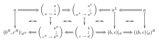
4. A first example
if foo.tex contains:
\documentclass{book}
\usepackage{proof}
\def\defded#1#2{\expandafter\def\csname ded-#1\endcsname{#2}}
\def\ded#1{\csname ded-#1\endcsname}
\begin{document}
\input foo.dnt
\def\<{\langle}
\def\>{\rangle}
%:*|->*\mapsto *
%:*->*\to *
%:*\\*\lambda *
%:*:*{:}*
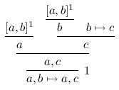
%:
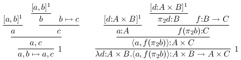
%: [a,b]^1 [d:A×B]^1
%: ------- ---------
%: [a,b]^1 b b|->c [d:A×B]^1 \pi_2d:B f:B->C
%: ------- ----------- --------- -------------------
%: a c a:A f(\pi_2b):C
%: -------------- -----------------------
%: a,c \<a,f(\pi_2b)\>:A×C
%: ---------1 --------------------------------1
%: a,b|->a,c \\d:A×B.\<a,f(\pi_2b)\>:A×B->A×C
%:
%: ^Atimes-DNC-notation ^Atimes-conventional
%:
$$\ded{Atimes-DNC-notation} \qquad \ded{Atimes-conventional}$$
\end{document}
|
then running "dednat4.lua foo.tex" and then "latex
foo.tex" will produce this,
because "dednat4.lua foo.tex" creates a a file foo.dnt
containing this:
\defded{Atimes-DNC-notation}{    % (find-fline "foo.tex" 27)
 \infer[{1}]{ \mathstrut a,b\mapsto a,c }{
  \infer{ \mathstrut a,c }{
   \infer{ \mathstrut a }{
    \mathstrut [a,b]^1 } &
   \infer{ \mathstrut c }{
    \infer{ \mathstrut b }{
     \mathstrut [a,b]^1 } &
    \mathstrut b\mapsto c } } } }

\defded{Atimes-conventional}{    % (find-fline "foo.tex" 27)
 \infer[{1}]{ \mathstrut \lambda d{:}A×B.\<a,f(\pi_2b)\>{:}A×B\to A×C }{
  \infer{ \mathstrut \<a,f(\pi_2b)\>{:}A×C }{
   \infer{ \mathstrut a{:}A }{
    \mathstrut [d{:}A×B]^1 } &
   \infer{ \mathstrut f(\pi_2b){:}C }{
    \infer{ \mathstrut \pi_2d{:}B }{
     \mathstrut [d{:}A×B]^1 } &
    \mathstrut f{:}B\to C } } } }
|
"\usepackage{proof}" loads Makoto Tatsuta's proof.sty package, which defines \infer. Dednat4's routines for tree output also support
Paul Taylor's "proofs" package, and inserting a line like
%L tex_tree_function = tex_tree_paultaylor |
in foo.tex anywhere before the
%: ^Atimes-DNC-notation ^Atimes-conventional |
line would make dednat4.lua spit out code for Paul Taylor's package instead.
5. Words
A word in dednat4's terminology (and in Forth terminology) is a sequence of non-whitespace characters, delimited by whitespace; the only characters that dednat4 considers as whitespace are " ", TAB, NL and CR (chars 32, 9, 10 and 13 respectively). The characters in the head of a line are removed before splitting it into words.
6. Everything about "%:" lines (and abbreviations)
The "%:" lines -- and also the "%D" lines, that we will
describe soon -- are processed word by word. As heads don't count to
form words, the line
%: ^Atimes-DNC-notation ^Atimes-conventional |
has two words, "^Atimes-DNC-notation" and "^Atimes-conventional". In "%:" lines only the words that start
with "^" are "active": "^Atimes-conventional" means "process
the deduction tree whose root node is two lines above the "^" and
output a block of TeX code of the form \defded{Atimes-conventional}{...} -- a definition for a deduction
called Atimes-conventional; the definition is invoked with \ded{Atimes-conventional}.
Deduction trees are made of "nodes" and "bars". Both nodes and bars are words. The TeX code for a node is obtained by expanding all the abbreviations in the word (the functions that do that are here). Note that the expansion of an abbreviation can contain spaces -- for example:
%:*|->*\mapsto * |
Bars are always words that start with either a sequence of one or more "-"s, or a sequence of one or more "="s (for double bars). The "rest" of the word of a bar, when it exists, has its abbreviations expanded and the resulting TeX code is typeset at the right of the bar.
A node can either have a bar above it or have nothing above it; a
bar can have any number of nodes above it. Here "above" means
"immediately above", and two words are only considered to be one above
the other when their horizontal ranges have at least one character in
common. In the example below the node "notabove" is not
considered to be above the bar.
%: abovethebar alsoabove notabove %: ===stuffattheright %: belowthebar |
7. A second example: categorical diagrams
The part of the source file that starts at this point implements the support for
"%D" lines. This part of dednat4 is a front-end for Michael
Barr's diagxy package, which
in its turn is a front-end for XYpic.
"%D" lines are processed one by one, and each word in them
(except the head) is parsed (the code for the parser starts here) and then is executed.
And there is a trick: some words advance the input pointer during
their execution, and process the text between the old "pos" and the
new "pos" in their own ways; usually they either read some words or
read everything up to the end of the line.
Here is our first example of code with "%D" lines. Suppose
that the file foo2.tex contains this:
\documentclass{book}
\input diagxy
\def\defdiag#1#2{\expandafter\def\csname diag-#1\endcsname{#2}}
\def\diag#1{\bfig\csname diag-#1\endcsname\efig}
\begin{document}
\input foo2.dnt
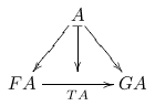
%D diagram T:F->G
%D 2Dx 100 +20 +20
%D 2D 100 A
%D 2D / - \
%D 2D / | \
%D 2D v v v
%D 2D +25 FA ------> GA
%D 2D TA
%L PP(nodes) -- Lua code: dump the table `nodes'
%D (( A FA -> A GA ->
%L PP(ds) -- Lua code: dump the table `ds'
%D FA GA -> .plabel= b TA
%D A FA GA midpoint |->
%D ))
%D enddiagram
$$\diag{T:F->G}$$
\end{document}
|
The first word parsed is "diagram". When it is executed it
reads the next word, "T:F->G", sets the name of the current
diagram to that, clears the tables that hold the catalog of known
nodes and arrows, and does a few other things; its code is here and here.
7.1. The 2D grid
Both "2Dx" and "2D" are words that parse everything to
the end of the line and treat what they read in their own ways - as
a grid with coordinates and nodes. Only columns that are below the
first character of a number in the "2Dx" line have a horizontal
coordinate; only lines that start with a number have a vertical
coordinate (these "numbers" can start with "+", that means "the
previous value plus this"). In the grid in foo2.tex only these six
positions, marked as `a', `b', `c', `d', `e', and `f' below, have
both a horizontal and a vertical coordinates; `e' has coordinates
(140, 125).
%D 2Dx 100 +20 +20 %D 2D 100 a b c %D 2D %D 2D %D 2D %D 2D +25 c d e %D 2D |
Some words in the grid in foo2.tex -- namely, "A", "FA",
"------>", and "GA", are over positions with both
coordinates; those words become names of nodes with those
coordinates. Most of the things that we drew on the grid are just
"decorations" that are ignored by "2D"; they are there just to
make the ASCII diagram look like a textual representation of the
real diagram. Note that the "------>", that in a sense is just
a decoration, is not ignored -- it becomes a node, but as
unused nodes don't show on the picture and don't generate TeX code,
we can ignore it.
After the grid in foo2.tex there's a Lua line with a command to dump the array of nodes; the source for PP is here, and the result (that is printed to stdout) is this, modulo whitespace:
{1={"noden"=1, "tag"="A", "x"=120, "y"=100},
 2={"noden"=2, "tag"="FA", "x"=100, "y"=125},
 3={"noden"=3, "tag"="------>", "x"=120, "y"=125},
 4={"noden"=4, "tag"="GA", "x"=140, "y"=125},
 "------>"={"noden"=3, "tag"="------>", "x"=120, "y"=125},
 "A"={"noden"=1, "tag"="A", "x"=120, "y"=100},
 "FA"={"noden"=2, "tag"="FA", "x"=100, "y"=125},
 "GA"={"noden"=4, "tag"="GA", "x"=140, "y"=125}
}
|
Note that entries in that table can be accessed either by a numeric
id (the "noden") or by the name of the node ("tag"); some of the
subtables are shared -- nodes[1] = nodes["A"] -- but the output
of PP doesn't make that explicit.
There's also a table called "arrows", but at this point it is
empty.
7.2. Building arrows
After that comes this code:
%D (( A FA -> A GA -> %L PP(ds) -- Lua code: dump the table `ds' %D FA GA -> .plabel= b TA %D A FA GA midpoint |-> %D )) |
Dednat4 has a data stack ("ds"; we will see a dump of it
soon), like Forth; it doesn't have a "return stack" like the one in
Forth, as we don't need subroutines in the obvious sense of the
term, at least not in the kernel; it's easy to define new words in
Lua, and usually that's enough.
"((" puts a value in an auxiliary stack, called "depths",
to remember how deep is the data stack at that point; in the next
lines we will put many new objects in the data stack, and the "))" will get rid of all these new objects: it will drop everything
above the stored depth. "((" and "))" help keeping the
data stack tidy.
"A" and "FA" put two nodes on the data stack; "->"
(the words for arrows are defined here) creates a new arrow, going
from "A" to "FA", and puts it both on the data stack
(after "A" and "FA") and on the list of arrows; the main
thing that "enddiagram" does is to output TeX code for all the
defined arrows, i.e., to draw them. This can only be done at the
end, because some words modify attributes of arrows: the code ".plabel= b TA", a few lines after that, adds a "label" and a
"position" to the arrow at the top of the stack: the text of the
label is "TA", and it is to be TeXed below the arrow.
When "PP(ds)" (in Lua) dumps the data stack what we see is
this, modulo whitespace:
{1={"arrown"=2, "from"=1, "shape"="->", "to"=4},
 2={"noden"=4, "tag"="GA", "x"=140, "y"=125},
 3={"noden"=1, "tag"="A", "x"=120, "y"=100},
 4={"arrown"=1, "from"=1, "shape"="->", "to"=2},
 5={"noden"=2, "tag"="FA", "x"=100, "y"=125},
 6={"noden"=1, "tag"="A", "x"=120, "y"=100}
}
|
A full description of the "node" and "arrow" structures can be
found here; arrows have many
optional fields. Note that the top of the stack is ds[1].
The only other new thing in this diagram is "midpoint". It is
defined here, and it takes the two nodes
at the top of the stack and replaces them (on the stack only!) by a
new node, lying halfway between them.
We have already described "))"; in this case it makes the depth
of ds go back to zero. After it "enddiagram" appends this to
foo2.dnt,
\defdiag{T:F->G}{    % (find-fline "foo2.tex" 9)
  \morphism(300,0)/->/<-300,-375>[{A}`{FA};{}]
  \morphism(300,0)/->/<300,-375>[{A}`{GA};{}]
  \morphism(0,-375)|b|/->/<600,0>[{FA}`{GA};{TA}]
  \morphism(300,0)/|->/<0,-375>[{A}`{\phantom{O}};{}]
}
|
And TeX typesets it into this:
7.3. More tricks for 2D diagrams
(Describe how to use "@" to refer to the elements pushed on the
stack after the last "((", how to use ".tex" and ".TeX" to have
several nodes with the same TeX text; also: other "shapes" of floating
arrows (=>, for example), "place" and the pullback symbol;
discuss the source code of the BCC diagram below; discuss the
extensions in experimental.lua)
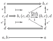
7.4. A bigger diagram
The diagram below - the Beck-Chevalley condition in a certain notation -
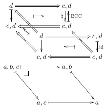
was produced by this code:
%D diagram LCCC-BCC
%D 2Dx         100     +30        +25      +30
%D 2D  100   {}d ===============> c,d{}
%D 2D          - /\               - ^
%D 2D          |  \\   |->        | |\BCC
%D 2D          v   \\             v -
%D 2D  +20  {}c,d <=\\=========== c,d{}{}
%D 2D           /\   \\             /\
%D 2D  +10       \\    d ===============> c,d{{}}
%D 2D             \\   -              \\   -
%D 2D              \\  |       <-|     \\  |\id
%D 2D               \\ v                \\ v
%D 2D  +20            c,d <============== c,d{{}}{}
%D 2D
%D 2D  +10     a,b,c |----------> a,b
%D 2D              -  _|              -
%D 2D               \                  \
%D 2D                v                  v
%D 2D  +35            a,c |--------------> a
%D 2D
%D ((  {}d      c,d{}		 # 0   1
%D    {}c,d     c,d{}{}	         # 2   3
%D           d        c,d{{}}    #   4   5
%D          c,d       c,d{{}}{}  #   6   7
%D    @ 0 @ 1 =>
%D    @ 0 @ 2 |-> @ 1 @ 3 |-> sl_ .plabel= l \natural
%D                @ 1 @ 3 <-| sl^ .plabel= r \mathrm{BCC}
%D            @ 0 @ 3 harrownodes nil 20 nil |->
%D    @ 2 @ 3 <=
%D    @ 0 @ 4 <=  @ 2 @ 6 <=  @ 3 @ 7 <=
%D    @ 0 @ 2 midpoint @ 4 @ 6 midpoint dharrownodes nil 14 nil <-|
%D    @ 4 @ 5 =>  @ 4 @ 6 |-> @ 5 @ 7 |-> .plabel= r \mathrm{id}
%D            @ 4 @ 7 harrownodes nil 20 nil <-|
%D    @ 6 @ 7 <=
%D ))
%D (( a,b,c     a,b
%D          a,c     a
%D    @ 0 @ 1 |->  @ 0 @ 2 |->  @ 1 @ 3 |->  @ 2 @ 3 |->
%D    @ 0 relplace 15 7 \pbsymbol{7}
%D ))
|
8. Help needed (mainly on xypic features that I don't understand)
In the section 4.6 ("Mixing XY-pic code") of diagxy manual there's a technique for drawing arrows whose paths are neither segments nor splines... it should be possible to use that to draw arrows whose paths are made of lines and arcs of circles, but I don't have any idea how... I find XY-pic far too difficult. 8-(
9. More examples
(This section was just copied from my math page...)
My PhD thesis included lots of hairy categorical diagrams, and I ended up writing a LaTeX preprocessor in Lua to help me typeset them. Currently (March 2005) I'm trying to pack that preprocessor and document it; its README is still horribly incomplete. The source code for the examples below is here.
|
|||||
|
|
|
|||